Styles, classes, labels and heatmaps

Every layer has a style. Select the layer and choose Layer → Style… (or Actions → Style… next to the layer). Changes show on the map and in the legend immediately; Undo reverts them.

Four ways to colour a layer

• Single colour — every feature looks the same.
• Categories (by value) — one colour per value of a field, for example zone = residential, mixed, industrial. Up to 60 categories; each colour can be changed.
• Classes (choropleth) — a number field is split into 2–12 classes, coloured along a ramp from light to dark.
• Heatmap — for point layers only: a density surface instead of single points.

Classes: which method?

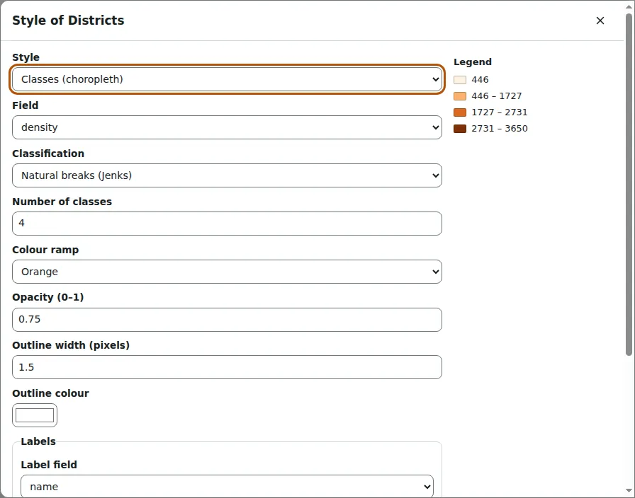
Open Town districts (choropleth) and the style of Districts. It colours the field density in four classes with Natural breaks (Jenks).

• Equal interval splits the range into steps of the same size. Easy to read, but one outlier can leave most classes empty.
• Quantile puts the same number of features in each class. Good for rankings; very different values can end up in the same class.
• Natural breaks (Jenks) finds the breaks that keep values within a class as close as possible (Fisher's exact method). Good for data with clusters.

The legend lists the class limits. When a field has fewer different values than classes, GISela uses one class per value.

Symbols and labels

Point layers have a symbol — circle, square, triangle, diamond, star or cross — and a size in pixels. Lines and polygon outlines have a width; polygons also have an outline colour. Opacity makes a layer see-through, which helps when layers overlap.

Under Labels, choose a field to write next to every feature, with a size, a colour and a white halo that keeps text readable on any background. Labels are drawn in the map, the print layout and SVG and PNG exports.

Heatmaps

Open Bird sightings heatmap. The 240 sightings are drawn as a density surface: every point spreads its weight over a radius (here 36 pixels) with a smooth quartic kernel, and the sums are coloured from yellow to dark red. With Weight field set to count, a sighting of twelve birds counts twelve times.

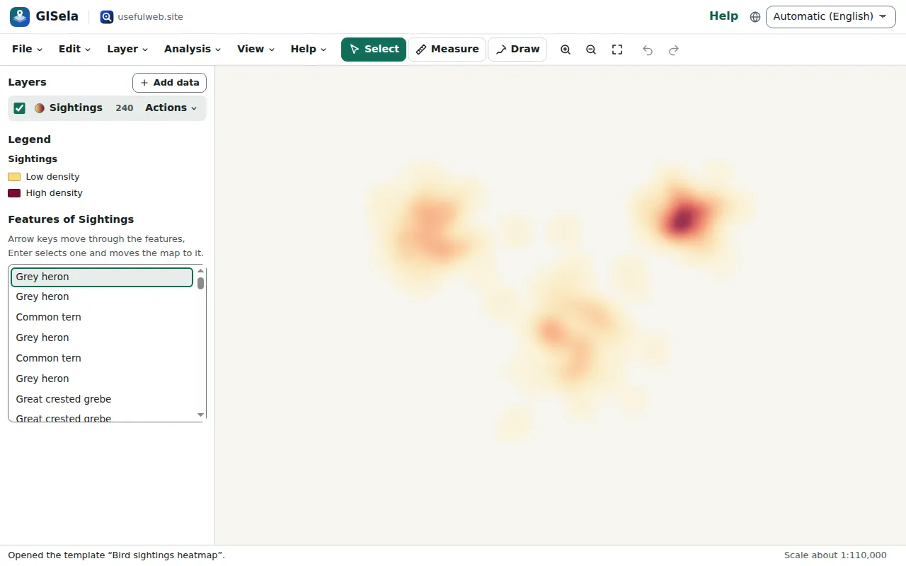
The radius is in screen pixels, so the surface looks the same at every zoom level and the hot spots stay visible when you zoom out. To see the individual sightings, switch the style to Single colour or Categories by species, or open the attribute table.